Artificial neural networks are statistical learning models, inspired by biological neural networks (central nervous systems, such as the brain), that are used in machine learning. These networks are represented as systems of interconnected “neurons”, which send messages to each other. The connections within the network can be systematically adjusted based on inputs and outputs, making them ideal for supervised learning.

Neural networks can be intimidating, especially for people with little experience in machine learning and cognitive science! However, through code, this tutorial will explain how neural networks operate. By the end, you will know how to build your own flexible, learning network, similar to Mind.

The only prerequisites are having a basic understanding of JavaScript, high-school Calculus, and simple matrix operations. Other than that, you don’t need to know anything. Have fun!

Understanding the Mind

A neural network is a collection of “neurons” with “synapses” connecting them. The collection is organized into three main parts: the input layer, the hidden layer, and the output layer. Note that you can have n hidden layers, with the term “deep” learning implying multiple hidden layers.

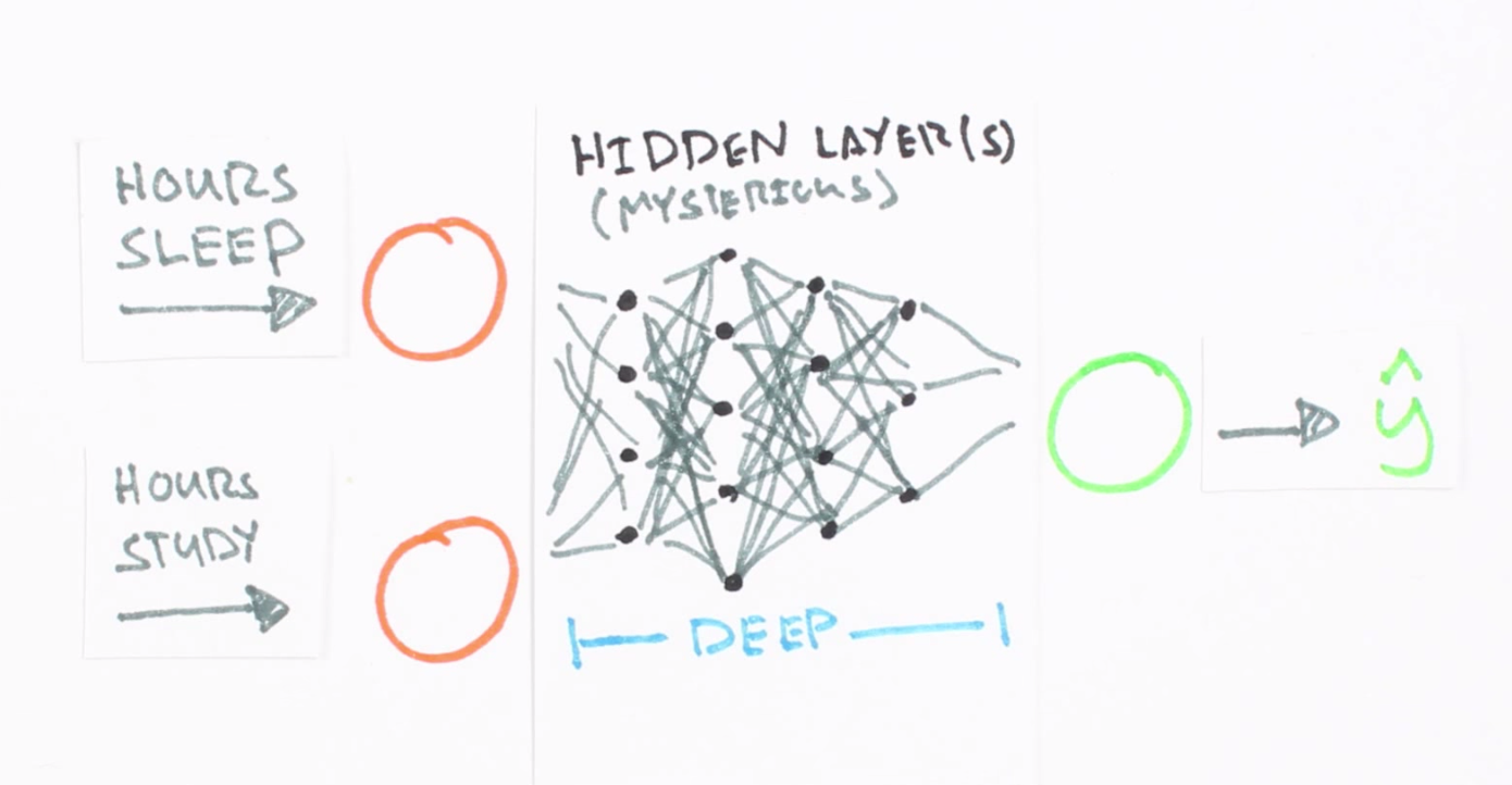
Screenshot taken from this great introductory video, which trains a neural network to predict a test score based on hours spent studying and sleeping the night before.

Hidden layers are necessary when the neural network has to make sense of something really complicated, contextual, or non obvious, like image recognition. The term “deep” learning came from having many hidden layers. These layers are known as “hidden”, since they are not visible as a network output. Read more about hidden layers here and here.

The circles represent neurons and lines represent synapses. Synapses take the input and multiply it by a “weight” (the “strength” of the input in determining the output). Neurons add the outputs from all synapses and apply an activation function.

Training a neural network basically means calibrating all of the “weights” by repeating two key steps, forward propagation and back propagation.

Since neural networks are great for regression, the best input data are numbers (as opposed to discrete values, like colors or movie genres, whose data is better for statistical classification models). The output data will be a number within a range like 0 and 1 (this ultimately depends on the activation function—more on this below).

In forward propagation, we apply a set of weights to the input data and calculate an output. For the first forward propagation, the set of weights is selected randomly.

In back propagation, we measure the margin of error of the output and adjust the weights accordingly to decrease the error.

Neural networks repeat both forward and back propagation until the weights are calibrated to accurately predict an output.

Next, we’ll walk through a simple example of training a neural network to function as an “Exclusive or” (“XOR”) operation to illustrate each step in the training process.

Forward Propagation

Note that all calculations will show figures truncated to the thousandths place.

The XOR function can be represented by the mapping of the below inputs and outputs, which we’ll use as training data. It should provide a correct output given any input acceptable by the XOR function.

input | output
--------------
0, 0  | 0
0, 1  | 1
1, 0  | 1
1, 1  | 0

Let’s use the last row from the above table, (1, 1) => 0, to demonstrate forward propagation:

Note that we use a single hidden layer with only three neurons for this example.

We now assign weights to all of the synapses. Note that these weights are selected randomly (based on Gaussian distribution) since it is the first time we’re forward propagating. The initial weights will be between 0 and 1, but note that the final weights don’t need to be.

We sum the product of the inputs with their corresponding set of weights to arrive at the first values for the hidden layer. You can think of the weights as measures of influence the input nodes have on the output.

1 * 0.8 + 1 * 0.2 = 1
1 * 0.4 + 1 * 0.9 = 1.3
1 * 0.3 + 1 * 0.5 = 0.8

We put these sums smaller in the circle, because they’re not the final value:

To get the final value, we apply the activation function to the hidden layer sums. The purpose of the activation function is to transform the input signal into an output signal and are necessary for neural networks to model complex non-linear patterns that simpler models might miss.

There are many types of activation functions—linear, sigmoid, hyperbolic tangent, even step-wise. To be honest, I don’t know why one function is better than another.

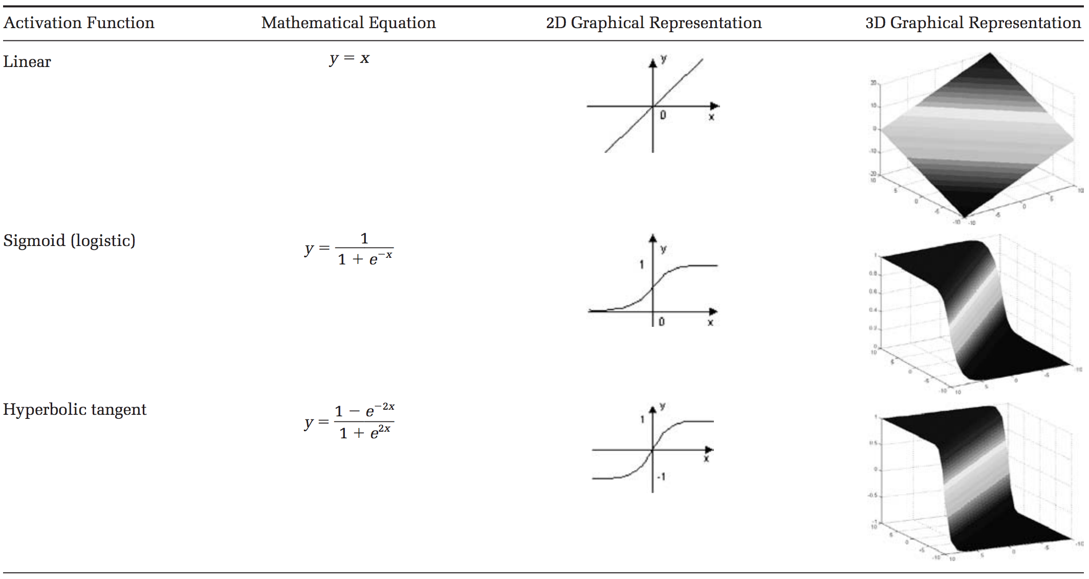
Table taken from this paper.

For our example, let’s use the sigmoid function for activation. The sigmoid function looks like this, graphically:

And applying S(x) to the three hidden layer sums, we get:

S(1.0) = 0.73105857863
S(1.3) = 0.78583498304
S(0.8) = 0.68997448112

We add that to our neural network as hidden layer results:

Then, we sum the product of the hidden layer results with the second set of weights (also determined at random the first time around) to determine the output sum.

0.73 * 0.3 + 0.79 * 0.5 + 0.69 * 0.9 = 1.235

..finally we apply the activation function to get the final output result.

S(1.235) = 0.7746924929149283

This is our full diagram:

Because we used a random set of initial weights, the value of the output neuron is off the mark; in this case by +0.77 (since the target is 0). If we stopped here, this set of weights would be a great neural network for inaccurately representing the XOR operation.

Let’s fix that by using back propagation to adjust the weights to improve the network!

Back Propagation

To improve our model, we first have to quantify just how wrong our predictions are. Then, we adjust the weights accordingly so that the margin of errors are decreased.

Similar to forward propagation, back propagation calculations occur at each “layer”. We begin by changing the weights between the hidden layer and the output layer.

Calculating the incremental change to these weights happens in two steps: 1) we find the margin of error of the output result (what we get after applying the activation function) to back out the necessary change in the output sum (we call this delta output sum) and 2) we extract the change in weights by multiplying delta output sum by the hidden layer results.

The output sum margin of error is the target output result minus the calculated output result:

And doing the math:

Target = 0
Calculated = 0.77
Target - calculated = -0.77

To calculate the necessary change in the output sum, or delta output sum, we take the derivative of the activation function and apply it to the output sum. In our example, the activation function is the sigmoid function.

To refresh your memory, the activation function, sigmoid, takes the sum and returns the result:

So the derivative of sigmoid, also known as sigmoid prime, will give us the rate of change (or “slope”) of the activation function at the output sum:

Since the output sum margin of error is the difference in the result, we can simply multiply that with the rate of change to give us the delta output sum:

Conceptually, this means that the change in the output sum is the same as the sigmoid prime of the output result. Doing the actual math, we get:

Delta output sum = S'(sum) * (output sum margin of error)
Delta output sum = S'(1.235) * (-0.77)
Delta output sum = -0.13439890643886018

Here is a graph of the Sigmoid function to give you an idea of how we are using the derivative to move the input towards the right direction. Note that this graph is not to scale.

Now that we have the proposed change in the output layer sum (-0.13), let’s use this in the derivative of the output sum function to determine the new change in weights.

As a reminder, the mathematical definition of the output sum is the product of the hidden layer result and the weights between the hidden and output layer:

The derivative of the output sum is:

..which can also be represented as:

This relationship suggests that a greater change in output sum yields a greater change in the weights; input neurons with the biggest contribution (higher weight to output neuron) should experience more change in the connecting synapse.

Let’s do the math:

hidden result 1 = 0.73105857863
hidden result 2 = 0.78583498304
hidden result 3 = 0.68997448112

Delta weights = delta output sum / hidden layer results
Delta weights = -0.1344 / [0.73105, 0.78583, 0.69997]
Delta weights = [-0.1838, -0.1710, -0.1920]

old w7 = 0.3
old w8 = 0.5
old w9 = 0.9

new w7 = 0.1162
new w8 = 0.329
new w9 = 0.708

To determine the change in the weights between the input and hidden layers, we perform the similar, but notably different, set of calculations. Note that in the following calculations, we use the initial weights instead of the recently adjusted weights from the first part of the backward propagation.

Remember that the relationship between the hidden result, the weights between the hidden and output layer, and the output sum is:

Instead of deriving for output sum, let’s derive for hidden result as a function of output sum to ultimately find out delta hidden sum:

Also, remember that the change in the hidden result can also be defined as:

Let’s multiply both sides by sigmoid prime of the hidden sum:

All of the pieces in the above equation can be calculated, so we can determine the delta hidden sum:

Delta hidden sum = delta output sum / hidden-to-outer weights * S'(hidden sum)
Delta hidden sum = -0.1344 / [0.3, 0.5, 0.9] * S'([1, 1.3, 0.8])
Delta hidden sum = [-0.448, -0.2688, -0.1493] * [0.1966, 0.1683, 0.2139]
Delta hidden sum = [-0.088, -0.0452, -0.0319]

Once we get the delta hidden sum, we calculate the change in weights between the input and hidden layer by dividing it with the input data, (1, 1). The input data here is equivalent to the hidden results in the earlier back propagation process to determine the change in the hidden-to-output weights. Here is the derivation of that relationship, similar to the one before:

Let’s do the math:

input 1 = 1
input 2 = 1

Delta weights = delta hidden sum / input data
Delta weights = [-0.088, -0.0452, -0.0319] / [1, 1]
Delta weights = [-0.088, -0.0452, -0.0319, -0.088, -0.0452, -0.0319]

old w1 = 0.8
old w2 = 0.4
old w3 = 0.3
old w4 = 0.2
old w5 = 0.9
old w6 = 0.5

new w1 = 0.712
new w2 = 0.3548
new w3 = 0.2681
new w4 = 0.112
new w5 = 0.8548
new w6 = 0.4681

Here are the new weights, right next to the initial random starting weights as comparison:

old         new
-----------------
w1: 0.8     w1: 0.712
w2: 0.4     w2: 0.3548
w3: 0.3     w3: 0.2681
w4: 0.2     w4: 0.112
w5: 0.9     w5: 0.8548
w6: 0.5     w6: 0.4681
w7: 0.3     w7: 0.1162
w8: 0.5     w8: 0.329
w9: 0.9     w9: 0.708

Once we arrive at the adjusted weights, we start again with forward propagation. When training a neural network, it is common to repeat both these processes thousands of times (by default, Mind iterates 10,000 times).

And doing a quick forward propagation, we can see that the final output here is a little closer to the expected output:

Through just one iteration of forward and back propagation, we’ve already improved the network!!

Check out this short video for a great explanation of identifying global minima in a cost function as a way to determine necessary weight changes.

If you enjoyed learning about how neural networks work, check out Part Two of this post to learn how to build your own neural network.